Preference Elicitation Task

Try the Demo

In this task, participants express their relative preferences among a set of stimulus options by allocating votes or weights. On each trial, multiple stimuli (images, text, videos, etc.) are displayed simultaneously, and participants can click to add votes or right-click to remove votes from each option. The relative weight of each option is visualized as a vertical bar above the stimulus, providing immediate visual feedback of the preference distribution.

This task implements various preference elicitation paradigms commonly used in behavioral economics, decision-making research, and voting systems. Different constraint types allow researchers to model scenarios ranging from unconstrained ratings to budget allocation, quadratic voting, and ranked preferences. The flexible constraint system enables investigation of preference structures under different decision contexts¹².

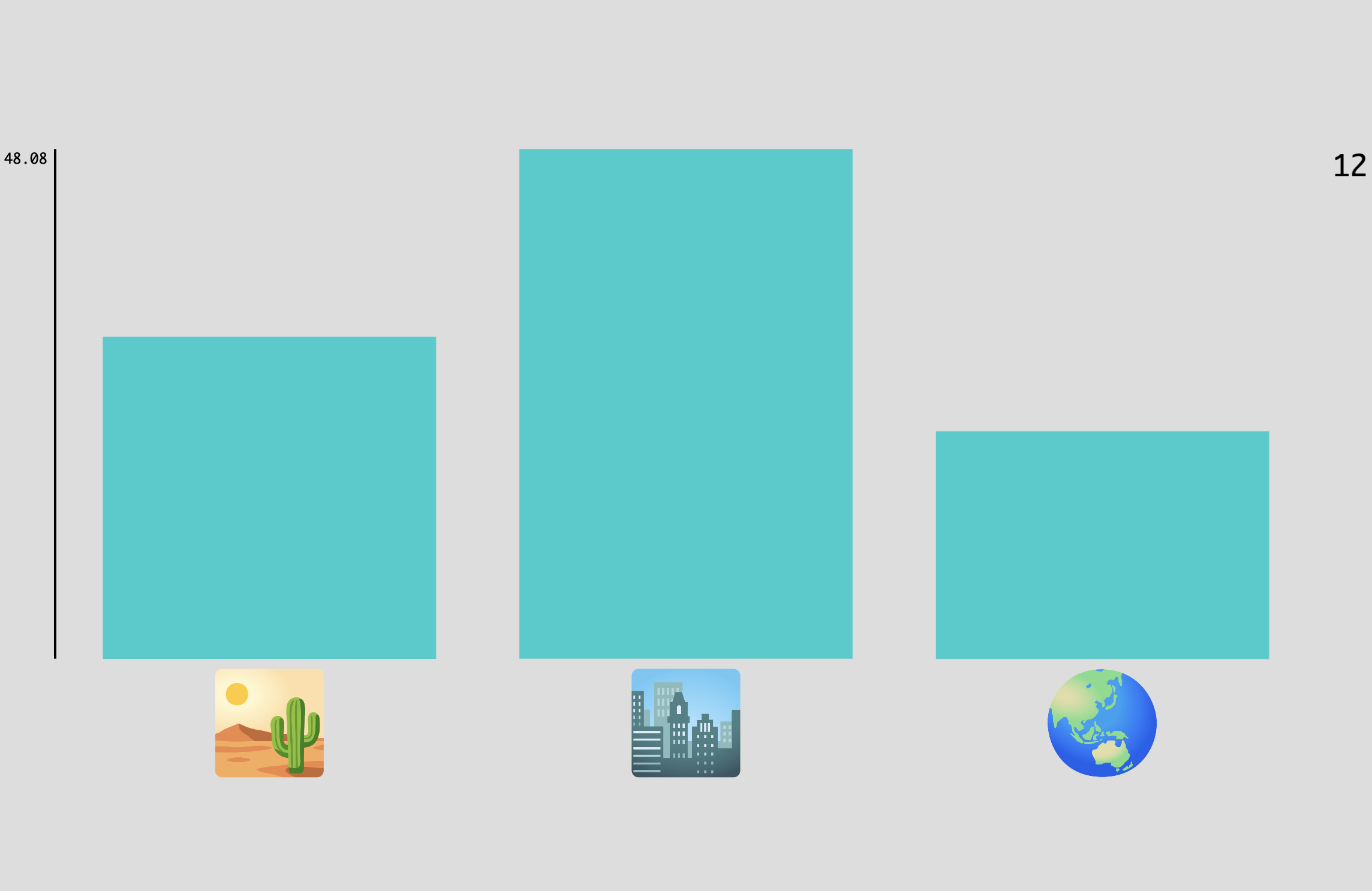
Example Preference Elicitation task showing multiple stimulus options with voting bars above each option. Participants allocate votes by clicking to increase or right-clicking to decrease the height of each bar.

Quick Start

1. Create or open an experiment from your Dashboard
2. Click Add task and select "Preference Elicitation"
3. Select a stimulus set with the options you want participants to evaluate
4. Choose a constraint type that matches your research question (see below)
5. Preview your experiment to verify the voting interface

New to Meadows? See the Getting Started guide for a complete walkthrough.

Alternative tasks

• Use an Order Sort task for simple ranking without vote allocation.
• Use a Circular Matching task for matching stimuli to a reference in a perceptual similarity task.
• Use a Stimulus Form task with rating scales for independent ratings of each stimulus.
• Use a Triplet Choice task for pairwise comparisons to infer preference rankings.

Constraint Types

The constraint type fundamentally changes how votes interact and what preference structure is captured:

No Constraint

Each option can be voted on independently with no interaction between options. Each vote always has value 1. This is suitable for:

• Binary probability elicitation: Each option receives independent ratings
• Range voting: Participants rate options on independent scales
• Separate evaluations: When options are not competing for limited resources

L0 Constraint

Implements k-hot selection where each option is either selected (vote = 1) or deselected (vote = 0). Only the selected subset matters, not the number of votes. Useful for:

• Subset selection: Choose which options meet a criterion
• Binary categorization: Classify stimuli into "chosen" vs "not chosen"

L1 Constraint

All options' weights sum to a fixed total value (set by displayed_total parameter). This is the classic budget constraint. Applications include:

• Probability distributions: Weights sum to 1.0 or 100%
• Resource allocation: Distribute a fixed budget across options
• Portfolio allocation: Divide investment across alternatives
• Attention allocation: Model limited attentional resources

L2 Constraint

Similar to L1, but additional votes have diminishing marginal value following a quadratic cost function. Each additional vote for an option costs more than the previous one². This models:

• Quadratic voting: Each vote costs the square of the vote number
• Quadratic funding: Democratic funding mechanisms
• Preference intensity: More natural expression of preference strength

Rank Constraint (No Ties)

Each vote switches an option's rank with the next highest-ranked option, creating a strict ordering. Useful for:

• Ranked-choice voting: Establish clear preference orderings
• Priority ranking: Determine sequential preferences
• Tournament rankings: Where ties are not allowed

Rank Constraint (With Ties)

Similar to rank constraint but allows multiple options to share the same rank. This enables:

• Flexible rankings: When some options are equally preferred
• Grouped preferences: Cluster options into preference tiers

Parameters

Customize the task by changing these on the Parameters tab of the task.

General Interface settings

Customize the instruction at the top of the page, as well as toolbar buttons. These apply to most task types on Meadows.

Instruction hint

Text that you can display during the task at the top of the page.

Extended instruction

A longer instruction that only appears if the participant hovers their mouse cursor over the hint.

Hint size

Whether to display the instruction, or hide it, and what font size to use.

Fullscreen button

Whether to display a button in the bottom toolbar that participants can use to switch fullscreen mode on and off.

Voting Configuration

Configure how votes are allocated and constrained.

Constraint

How votes for individual options affect others. Options:

• No Constraint: Independent voting, no interaction between options
• L0 Constraint: Binary selection (selected/not selected)
• L1 Constraint: Weights sum to a fixed total (budget constraint)
• L2 Constraint: Quadratic cost for additional votes
• Rank Constraint (No ties): Strict preference ordering
• Rank Constraint (With ties): Ranking with tied ranks allowed

Default: No Constraint.

Displayed Total

The total value that votes sum to. Only applies when using L1 or L2 constraints. Default: 100. Valid range: 1 to 3000.

Limited Votes

Enable to limit the total number of votes available to the participant. When enabled, a vote counter is displayed in the top-right corner. Default: unchecked.

Number of Votes

How many votes the participant can allocate in total. Only applies when Limited Votes is enabled. Default: 10. Valid range: 1 to 999.

Trial Configuration

Control the presentation of stimuli across trials.

Items per Trial

The number of stimulus options displayed simultaneously in each trial. Default: 2. Valid range: 1 to 10.

Note

This setting does not apply when using trial files to specify exact stimulus combinations.

Adaptive Order

When enabled, options are automatically reordered on screen based on their current rank (highest-ranked at top). By default, options remain in their original presentation order. Default: unchecked.

Data

For general information about the various structures and file formats that you can download for your data see Downloads.

Annotations

Trial-wise "annotations" (table rows), with one row per trial. Columns:

• trial - numerical index of the trial
• time_trial_start - timestamp when the trial began (seconds since 1/1/1970)
• time_trial_end - timestamp when the participant submitted the trial (seconds since 1/1/1970)
• stim1_id, stim2_id, ... - meadows internal IDs of the stimuli presented (one column per item)
• stim1_name, stim2_name, ... - filenames of the stimuli as uploaded (one column per item)
• label - the allocated votes separated by underscores, e.g., 5_3_2 for three options receiving 5, 3, and 2 votes respectively

Analysis

Basic Vote Distribution Analysis

Extract and analyze how votes were distributed across options.

PythonR

import pandas as pd
import numpy as np
import matplotlib.pyplot as plt

# Load the annotations data
df = pd.read_csv('Meadows_myExperiment_v1_annotations.csv')

# Parse votes from the label column
df['votes'] = df['label'].str.split('_')
df['votes'] = df['votes'].apply(lambda x: [int(v) for v in x])

# Calculate trial duration in seconds
df['duration_sec'] = df['time_trial_end'] - df['time_trial_start']

# Get number of options per trial
df['n_options'] = df['votes'].apply(len)

# Calculate vote statistics per trial
df['total_votes'] = df['votes'].apply(sum)
df['max_votes'] = df['votes'].apply(max)
df['min_votes'] = df['votes'].apply(min)
df['vote_range'] = df['max_votes'] - df['min_votes']

# Calculate vote concentration (Gini coefficient)
def gini(votes):
    votes = sorted(votes)
    n = len(votes)
    if sum(votes) == 0:
        return 0
    cumsum = np.cumsum(votes)
    return (2 * np.sum((np.arange(1, n+1) - 1) * votes)) / (n * sum(votes)) - (n - 1) / n

df['vote_concentration'] = df['votes'].apply(gini)

# Summary statistics
print("Vote Distribution Summary:")
print(f"Average total votes per trial: {df['total_votes'].mean():.2f}")
print(f"Average vote concentration (Gini): {df['vote_concentration'].mean():.3f}")
print(f"Average trial duration: {df['duration_sec'].mean():.2f}s")

# Plot vote distribution across trials
fig, axes = plt.subplots(2, 2, figsize=(12, 10))

# Histogram of total votes
axes[0, 0].hist(df['total_votes'], bins=20, edgecolor='black')
axes[0, 0].set_xlabel('Total Votes per Trial')
axes[0, 0].set_ylabel('Frequency')
axes[0, 0].set_title('Distribution of Total Votes')

# Vote concentration
axes[0, 1].hist(df['vote_concentration'], bins=20, edgecolor='black')
axes[0, 1].set_xlabel('Vote Concentration (Gini)')
axes[0, 1].set_ylabel('Frequency')
axes[0, 1].set_title('Vote Concentration Across Trials')

# Trial duration
axes[1, 0].hist(df['duration_sec'], bins=20, edgecolor='black')
axes[1, 0].set_xlabel('Trial Duration (seconds)')
axes[1, 0].set_ylabel('Frequency')
axes[1, 0].set_title('Trial Duration Distribution')

# Vote range
axes[1, 1].hist(df['vote_range'], bins=20, edgecolor='black')
axes[1, 1].set_xlabel('Vote Range (Max - Min)')
axes[1, 1].set_ylabel('Frequency')
axes[1, 1].set_title('Vote Range Distribution')

plt.tight_layout()
plt.show()

library(tidyverse)

# Load the annotations data
df <- read_csv('Meadows_myExperiment_v1_annotations.csv')

# Parse votes from label column
df <- df %>%
  mutate(
    votes = str_split(label, '_'),
    votes = map(votes, as.integer),
    duration_sec = time_trial_end - time_trial_start,
    n_options = map_int(votes, length),
    total_votes = map_int(votes, sum),
    max_votes = map_int(votes, max),
    min_votes = map_int(votes, min),
    vote_range = max_votes - min_votes
  )

# Calculate Gini coefficient for vote concentration
gini <- function(votes) {
  votes <- sort(votes)
  n <- length(votes)
  if (sum(votes) == 0) return(0)
  cumsum_votes <- cumsum(votes)
  (2 * sum((seq_len(n) - 1) * votes)) / (n * sum(votes)) - (n - 1) / n
}

df <- df %>%
  mutate(vote_concentration = map_dbl(votes, gini))

# Summary statistics
cat("Vote Distribution Summary:\n")
df %>%
  summarise(
    avg_total_votes = mean(total_votes),
    avg_concentration = mean(vote_concentration),
    avg_duration = mean(duration_sec)
  ) %>%
  print()

# Plot vote distributions
p1 <- ggplot(df, aes(x = total_votes)) +
  geom_histogram(bins = 20, fill = 'steelblue', color = 'black') +
  labs(x = 'Total Votes per Trial', y = 'Frequency',
       title = 'Distribution of Total Votes') +
  theme_minimal()

p2 <- ggplot(df, aes(x = vote_concentration)) +
  geom_histogram(bins = 20, fill = 'steelblue', color = 'black') +
  labs(x = 'Vote Concentration (Gini)', y = 'Frequency',
       title = 'Vote Concentration Across Trials') +
  theme_minimal()

# Display plots
library(patchwork)
p1 + p2

Stimulus Preference Aggregation

Aggregate votes across trials to determine overall stimulus preferences.

PythonRSpreadsheet

import pandas as pd
import matplotlib.pyplot as plt

# Load the annotations data
df = pd.read_csv('Meadows_myExperiment_v1_annotations.csv')

# Parse votes
df['votes'] = df['label'].str.split('_').apply(lambda x: [int(v) for v in x])

# Find all stimulus columns
stim_id_cols = [col for col in df.columns if col.startswith('stim') and col.endswith('_id')]
stim_name_cols = [col for col in df.columns if col.startswith('stim') and col.endswith('_name')]

# Reshape data to long format with stimulus-vote pairs
records = []
for idx, row in df.iterrows():
    votes = row['votes']
    for i, (id_col, name_col) in enumerate(zip(stim_id_cols, stim_name_cols)):
        if i < len(votes) and pd.notna(row[id_col]):
            records.append({
                'stimulus_id': row[id_col],
                'stimulus_name': row[name_col],
                'votes': votes[i],
                'trial': row['trial']
            })

stim_df = pd.DataFrame(records)

# Aggregate votes per stimulus
stim_summary = stim_df.groupby(['stimulus_id', 'stimulus_name']).agg({
    'votes': ['sum', 'mean', 'std', 'count']
}).round(2)
stim_summary.columns = ['total_votes', 'mean_votes', 'std_votes', 'n_presentations']
stim_summary = stim_summary.reset_index().sort_values('total_votes', ascending=False)

print("\nStimulus Preference Ranking:")
print(stim_summary)

# Plot top stimuli by total votes
top_n = min(15, len(stim_summary))
plt.figure(figsize=(12, 6))
plt.barh(range(top_n), stim_summary['total_votes'].head(top_n))
plt.yticks(range(top_n), stim_summary['stimulus_name'].head(top_n))
plt.xlabel('Total Votes')
plt.title(f'Top {top_n} Most Preferred Stimuli')
plt.gca().invert_yaxis()
plt.tight_layout()
plt.show()

library(tidyverse)

# Load the annotations data
df <- read_csv('Meadows_myExperiment_v1_annotations.csv')

# Parse votes
df <- df %>%
  mutate(votes = str_split(label, '_'),
         votes = map(votes, as.integer))

# Find stimulus columns
stim_cols <- colnames(df) %>%
  str_subset('stim\\d+_(id|name)')

# Reshape to long format
stim_df <- df %>%
  select(trial, votes, starts_with('stim')) %>%
  pivot_longer(
    cols = starts_with('stim'),
    names_to = c('stim_num', 'type'),
    names_pattern = '(stim\\d+)_(id|name)',
    values_to = 'value'
  ) %>%
  pivot_wider(names_from = type, values_from = value) %>%
  mutate(stim_num = as.integer(str_extract(stim_num, '\\d+'))) %>%
  filter(!is.na(id)) %>%
  rowwise() %>%
  mutate(vote_value = votes[[stim_num]]) %>%
  ungroup()

# Aggregate by stimulus
stim_summary <- stim_df %>%
  group_by(stimulus_id = id, stimulus_name = name) %>%
  summarise(
    total_votes = sum(vote_value),
    mean_votes = mean(vote_value),
    std_votes = sd(vote_value),
    n_presentations = n(),
    .groups = 'drop'
  ) %>%
  arrange(desc(total_votes))

print(stim_summary)

# Plot top stimuli
top_n <- min(15, nrow(stim_summary))
stim_summary %>%
  head(top_n) %>%
  mutate(stimulus_name = fct_reorder(stimulus_name, total_votes)) %>%
  ggplot(aes(x = total_votes, y = stimulus_name)) +
  geom_col(fill = 'steelblue') +
  labs(x = 'Total Votes', y = NULL,
       title = paste('Top', top_n, 'Most Preferred Stimuli')) +
  theme_minimal()

For basic analysis in Excel or Google Sheets:

1. Open the Meadows_myExperiment_v1_annotations.csv file
2. Insert a new column after the label column
3. To extract the first stimulus's votes, use: =VALUE(LEFT(label, FIND("_", label)-1))
4. For the second stimulus: =VALUE(MID(label, FIND("_", label)+1, FIND("_", label, FIND("_", label)+1) - FIND("_", label)-1))
5. Create a pivot table with:
   • Rows: stim1_name (or other stimulus columns)
   • Values: Sum and Average of the extracted vote columns
6. Sort by total votes to see most preferred stimuli

References

---

1. Iyengar, G., Lee, J., & Campbell, M. (2001). Q-Eval: Evaluating multiple attribute items using queries. Proceedings of the 2001 ACM conference on Electronic commerce, 144-153. doi:10.1145/501158.501179 ↩

2. Quarfoot, D., von Kohorn, D., Slavin, K., Sutherland, R., Konar, E., & Still, K. (2017). Quadratic voting in the wild: Real people, real votes. Public Choice, 172(1-2), 283-303. doi:10.1007/s11127-017-0416-1 ↩↩