Match-to-Sample Task
In this task, participants are presented with a sample (target) stimulus alongside two alternative stimuli. The participant selects which of the two alternatives matches the sample by clicking on it. This task is a fundamental paradigm for studying learning, memory, discrimination, and concept formation.
The matching-to-sample paradigm has been extensively used in behavioral research since the 1960s1. Originally developed for operant conditioning studies, it has become a versatile tool for investigating perceptual matching, working memory, and conceptual similarity across diverse stimulus domains including visual, auditory, and abstract stimuli. The paradigm is particularly valuable because it provides a clear measure of whether participants can discriminate and match stimuli based on specific features or learned associations.
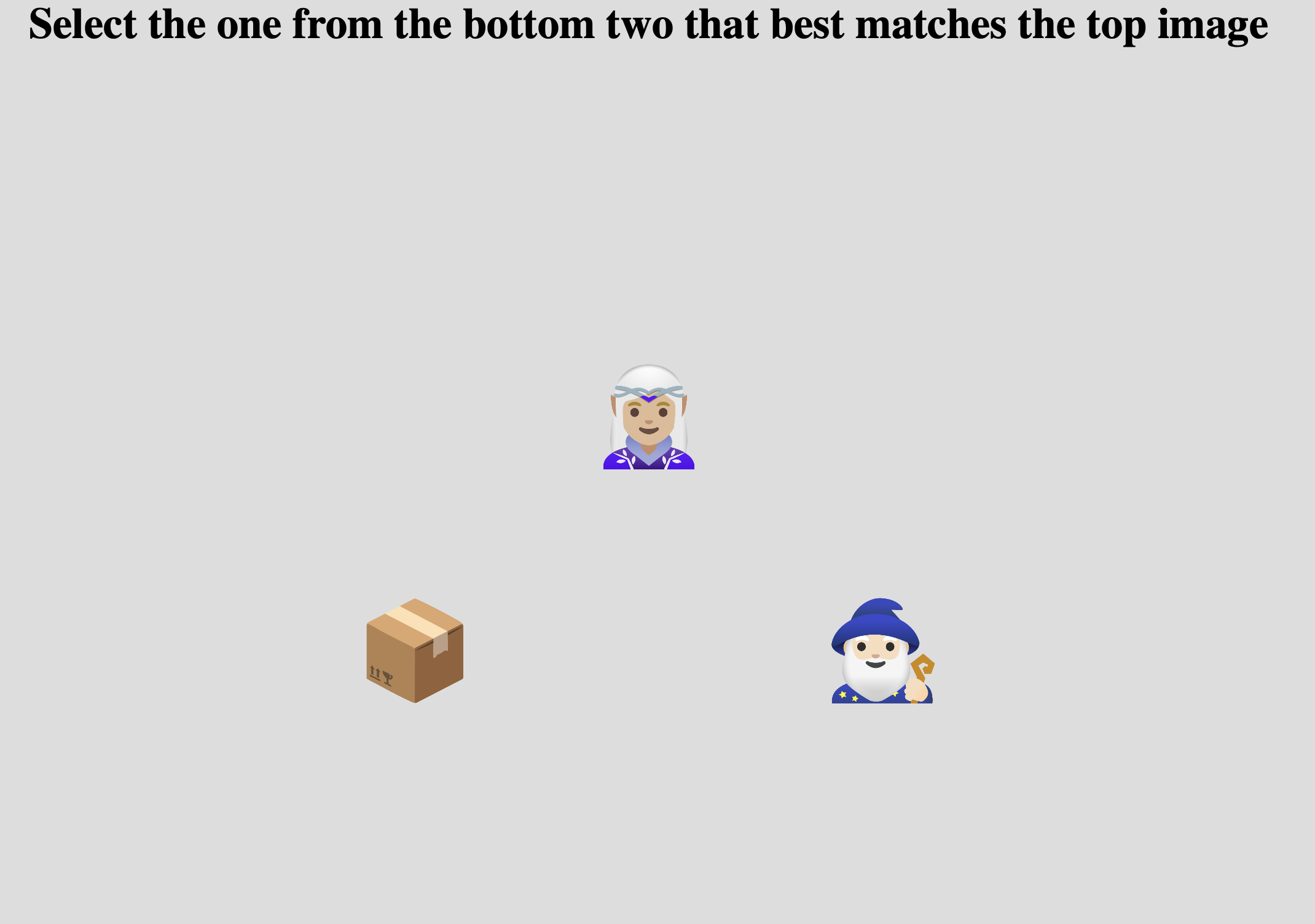
Example Match-to-Sample task showing a sample stimulus (top) with two alternatives below. The participant clicks on the matching alternative.
Quick Start
- Create or open an experiment from your Dashboard
- Click Add task and select "Match-to-Sample"
- Select a stimulus set with at least 2 stimuli
- Configure spatial layout and stimulus sizes
- Preview your experiment
New to Meadows? See the Getting Started guide for a complete walkthrough.
Alternative tasks
- Use a Triplet Choice task for odd-one-out judgments with three stimuli where all are clickable.
- Use a Discriminability task for same/different judgments between pairs of stimuli.
- Use a Circular Matching task for matching to a central reference from multiple arranged alternatives.
Parameters
Customize the task by changing these on the Parameters tab of the task.
General Interface settings
Customize the instruction at the top of the page, as well as toolbar buttons. These apply to most task types on Meadows.
Instruction hint-
Text that you can display during the task at the top of the page.
Extended instruction-
A longer instruction that only appears if the participant hovers their mouse cursor over the hint.
Tip
Make clear to participants what criterion they should use for matching. For example: "Click on the image that matches the one at the top" or "Select the stimulus that is most similar to the sample."
Hint size-
Whether to display the instruction, or hide it, and what font size to use.
Fullscreen button-
Whether to display a button in the bottom toolbar that participants can use to switch fullscreen mode on and off.
Trials and stimuli
Control the number of trials and how stimuli are combined into triplets.
Maximum Number Of Trials-
The number of trials will equal the total number of unique triplet combinations of stimuli, or this parameter, whichever is smaller. The task generates triplets by combining stimuli where one serves as the sample and two as alternatives. Default: 50. Must be between 1 and 1000.
Trial generation
Trials are generated by sampling triplets of stimuli. The first stimulus in each triplet serves as the sample, while the second and third are the alternatives. One of the alternatives will match the sample (either identical or from a matching category).
Blank Duration-
Duration in milliseconds to show a blank screen between trials. Set to 0 to turn this off. Default: 500 ms. Must be between 0 and 5000 ms.
Minimum Trial Duration-
The stimuli will be displayed for at least this duration (in milliseconds), even if a response was given earlier. This ensures participants view the stimuli for a minimum amount of time. Default: 0 ms. Must be between 0 and 10,000 ms.
Cannot Confirm Trial Until All Audio/Video Stimuli Have Finished-
If enabled, participants must wait for all audio or video stimuli to finish playing before they can confirm their selection. Default: False.
Wait Button Text-
Caption of the submit button when the trial is not ready yet (e.g., minimum duration not reached, or media still playing). Default: "wait..". Max 20 characters.
Spatial configuration
Options for customizing the layout and size of stimuli on the screen.
Layout-
How to arrange the stimuli on the screen. Options:
- Centered (default): All stimuli are spread out evenly with the sample at the top and the two alternatives centered below it. This provides balanced spacing.
- Justified: Stimuli are aligned with the edges of the screen. The sample is centered at the top, while alternatives are positioned at the bottom-left and bottom-right corners. This is most useful for large stimulus sizes to prevent overlap.
- Sample Justified, Alternatives Centered: The sample is justified (centered at top edge), while the two alternatives remain centered below. This provides a hybrid layout.
Item Size-
Height of the alternative stimuli. Default: 8.0. Must be between 0.2 and 40.0. The width is adapted according to the original aspect ratio of the stimulus.
Item Unit-
The unit to use for the size of the stimuli. Options:
- Percentage of the available width (default)
- Centimeters - requires participant calibration
- Visual angle in Degrees - requires participant calibration and distance measurement
See the documentation page "Dimensions, Units & Calibration" for more details.
Sample Size Ratio-
Adjust the size of the sample (target) stimulus by this factor relative to the alternative stimuli. For example, a value of 1.5 makes the sample 50% larger than the alternatives, while 0.5 makes it half the size. Default: 1.0 (same size). Must be between 0.1 and 10.0.
Example
With Item Size set to 8.0 and Sample Size Ratio set to 1.5, the alternatives will
have a height of 8.0 (in the chosen unit), while the sample will have a height of 12.0.
This can help visually distinguish the sample from the alternatives.
Visual feedback
Target Outline Thickness-
Width (in pixels) of the border displayed around the selected stimulus. Set to 0 for no outline. Default: 0. Must be between 0 and 50.
Target Outline Color-
Color of the border around the selected stimulus. Options: Red, Green, Blue, Black, White. Default: Red.
Data
For general information about the various structures and file formats that you can download for your data see Downloads.
Trial-wise "annotations" (table rows). Each row represents one trial. Columns:
taskName of the taskparticipationName of the experiment/participationtrialNumerical index of the trial (starting from 0)time_trial_startTimestamp when the trial was displayed (seconds since 1/1/1970)time_trial_responseTimestamp when the participant responded (seconds since 1/1/1970)stim1_idMeadows internal ID of the sample (target) stimulusstim1_nameFilename of the sample stimulus as uploadedstim2_idMeadows internal ID of the first alternative stimulusstim2_nameFilename of the first alternative as uploadedstim3_idMeadows internal ID of the second alternative stimulusstim3_nameFilename of the second alternative as uploadedlabelID of the stimulus that was selected by the participant
In the Tree structure, under the task object:
annotationsAn array with a key/value map for each trial:trialNumerical index of the trialstartTimestamp (epoch time) of the start of the trial, in seconds since 1/1/1970respTimestamp (epoch time) of the response, in seconds since 1/1/1970idsArray of three stimulus IDs: [sample, alternative1, alternative2]labelThe ID of the stimulus selected by the participant
stimuliArray of stimulus objects withidandnamefields
Analysis and Visualization
The match-to-sample task data can be analyzed to compute accuracy and reaction times, and to assess learning or discrimination performance across conditions.
Calculate Accuracy and Reaction Times
A response is correct when the participant selects the stimulus that matches the sample. This can be determined by comparing the selected stimulus ID with the sample ID (for identical matching) or by checking stimulus categories (for categorical matching).
import pandas as pd
import matplotlib.pyplot as plt

# Load the annotations data
df = pd.read_csv('Meadows_myExperiment_v1_annotations.csv')

# Calculate reaction time in milliseconds
df['rt_ms'] = (df['time_trial_response'] - df['time_trial_start']) * 1000

# Determine if response was correct
# For identical matching: check if selected stimulus matches sample
df['correct'] = (df['label'] == df['stim1_id']) | \
                (df['label'] == df['stim2_id']) & (df['stim2_id'] == df['stim1_id']) | \
                (df['label'] == df['stim3_id']) & (df['stim3_id'] == df['stim1_id'])

# Alternative: for categorical matching, you'd check if labels match
# df['correct'] = df['label'].str.contains(df['stim1_name'].str.split('_').str[0])

# Basic statistics
accuracy = df['correct'].mean() * 100
mean_rt = df['rt_ms'].mean()
mean_rt_correct = df[df['correct']]['rt_ms'].mean()
mean_rt_incorrect = df[~df['correct']]['rt_ms'].mean()

print(f"Overall accuracy: {accuracy:.1f}%")
print(f"Mean RT (all trials): {mean_rt:.2f} ms")
print(f"Mean RT (correct): {mean_rt_correct:.2f} ms")
print(f"Mean RT (incorrect): {mean_rt_incorrect:.2f} ms")

# Plot RT distributions for correct vs incorrect
fig, (ax1, ax2) = plt.subplots(1, 2, figsize=(12, 5))

ax1.hist(df[df['correct']]['rt_ms'], bins=30, alpha=0.7,
         label='Correct', color='green', edgecolor='black')
ax1.hist(df[~df['correct']]['rt_ms'], bins=30, alpha=0.7,
         label='Incorrect', color='red', edgecolor='black')
ax1.set_xlabel('Reaction Time (ms)')
ax1.set_ylabel('Frequency')
ax1.set_title('RT Distribution by Accuracy')
ax1.legend()

# Accuracy over trials (to see learning)
window = 10  # rolling window size
df['accuracy_rolling'] = df['correct'].rolling(window=window).mean()
ax2.plot(df['trial'], df['accuracy_rolling'])
ax2.axhline(y=0.5, color='gray', linestyle='--', label='Chance')
ax2.set_xlabel('Trial Number')
ax2.set_ylabel(f'Accuracy (rolling {window}-trial window)')
ax2.set_title('Learning Curve')
ax2.legend()

plt.tight_layout()
plt.show()
library(tidyverse)

# Load the annotations data
df <- read_csv('Meadows_myExperiment_v1_annotations.csv')

# Calculate reaction time in seconds
df <- df %>%
  mutate(
    rt_ms = (time_trial_response - time_trial_start) * 1000,
    # Determine correctness (for identical matching)
    correct = (label == stim1_id) |
              (label == stim2_id & stim2_id == stim1_id) |
              (label == stim3_id & stim3_id == stim1_id)
  )

# Summary statistics
df %>%
  summarise(
    accuracy = mean(correct) * 100,
    mean_rt = mean(rt_ms),
    median_rt = median(rt_ms),
    sd_rt = sd(rt_ms)
  )

# Statistics by accuracy
df %>%
  group_by(correct) %>%
  summarise(
    n = n(),
    mean_rt = mean(rt_ms),
    sd_rt = sd(rt_ms)
  )

# Plot RT by accuracy
ggplot(df, aes(x = correct, y = rt_ms, fill = correct)) +
  geom_boxplot() +
  scale_fill_manual(values = c("TRUE" = "green", "FALSE" = "red"),
                   labels = c("Incorrect", "Correct")) +
  labs(x = "Response Accuracy", y = "Reaction Time (ms)",
       title = "Reaction Times by Accuracy") +
  theme_minimal() +
  theme(legend.title = element_blank())
For basic analysis in Excel, Google Sheets, or LibreOffice Calc:
-
Calculate RT: In a new column, compute:
-
Determine accuracy: Create a column to check if the response matches:
Or for categorical matching: -
Calculate statistics:
- Mean accuracy:
=AVERAGE(correct_column) - Mean RT:
=AVERAGE(rt_column) -
Mean RT for correct:
=AVERAGEIF(correct_column, 1, rt_column) -
Create a pivot table to analyze accuracy by stimulus or trial block.
% Load the data
data = readtable('Meadows_myExperiment_v1_annotations.csv');

% Calculate reaction time in milliseconds
data.rt_ms = (data.time_trial_response - data.time_trial_start) * 1000;

% Determine correctness
data.correct = strcmp(data.label, data.stim1_id) | ...
               (strcmp(data.label, data.stim2_id) & strcmp(data.stim2_id, data.stim1_id)) | ...
               (strcmp(data.label, data.stim3_id) & strcmp(data.stim3_id, data.stim1_id));

% Calculate statistics
accuracy = mean(data.correct) * 100;
mean_rt = mean(data.rt_ms);
mean_rt_correct = mean(data.rt_ms(data.correct));
mean_rt_incorrect = mean(data.rt_ms(~data.correct));

fprintf('Overall accuracy: %.1f%%\n', accuracy);
fprintf('Mean RT (all): %.2f ms\n', mean_rt);
fprintf('Mean RT (correct): %.2f ms\n', mean_rt_correct);
fprintf('Mean RT (incorrect): %.2f ms\n', mean_rt_incorrect);

% Plot RT distributions
figure('Position', [100, 100, 1200, 500]);

subplot(1, 2, 1);
histogram(data.rt_ms(data.correct), 30, 'FaceColor', 'g', 'FaceAlpha', 0.7);
hold on;
histogram(data.rt_ms(~data.correct), 30, 'FaceColor', 'r', 'FaceAlpha', 0.7);
xlabel('Reaction Time (ms)');
ylabel('Frequency');
title('RT Distribution by Accuracy');
legend({'Correct', 'Incorrect'});

% Learning curve
subplot(1, 2, 2);
window = 10;
accuracy_rolling = movmean(double(data.correct), window);
plot(data.trial, accuracy_rolling, 'LineWidth', 2);
hold on;
yline(0.5, '--', 'Color', [0.5 0.5 0.5], 'LineWidth', 1.5);
xlabel('Trial Number');
ylabel(sprintf('Accuracy (rolling %d-trial window)', window));
title('Learning Curve');
legend({'Accuracy', 'Chance'}, 'Location', 'best');
References
-
Cumming, W. W., & Berryman, R. (1965). The complex discriminated operant: Studies of matching-to-sample and related problems. In D. I. Mostofsky (Ed.), Stimulus generalization (pp. 284-330). Stanford University Press. ↩